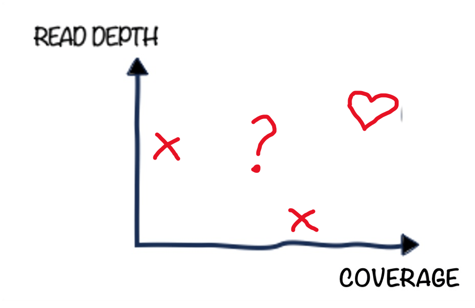
Two distinct key metrics can help you make sense of your sequencing experiments, if used correctly. But don’t fall into the misconception that these two can be used interchangeably (I fell for it, no judgment here): confuse sequencing coverage and read depth, and your analysis will suffer.
NOTE: this is the four instalment in my series on Common Misconceptions in Genomics (full list at the bottom).
THE TWO METRICS
When you describe your experiment in terms of coverage and read depth, you are essentially drawing a 2D plane and slapping your dataset(s) onto it.
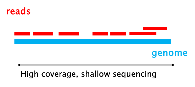
COVERAGE
The horizontal axis, it represents the “breadth” of your sequencing. This metric indicates what fraction of the genome was sequenced at least once.
The sequencing coverage is expressed as a percentage (%). Example: if one or more reads align to 90,000 bp of a 100,000 bp genome, the coverage is 90%.
High coverage is essential to produce a complete representation of the genome you have sequenced. It ensures that you have no blind spots, that is regions of unknown sequence.
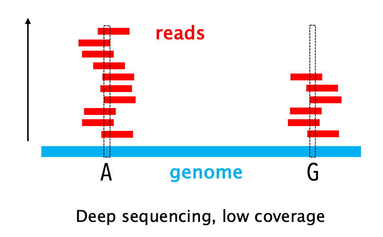
READ DEPTH
The vertical axis, it represents the “redundancy” of your sequencing. This metric counts how many times a specific base has been sequenced, that is how many individual reads overlap at that specific genetic coordinate.
The read depth is expressed as a multiplier (x). Example: if a stack of 1,000 reads covers a certain sequence, the read depth in that region is 1,000x.
High depth is crucial to produce an accurate representation of the genome, as stacking multiple reads enables you to distinguish a genuine genetic variant from a sequencing error.
DIFFERENT BUT RELATED
Now that another misconception in genomics is out of the way, it’s time for a twist: coverage and read depth are not independent. In fact, they’re mathematically linked. Your intuition is probably not shocked: the more you sequence a genome, the more likely you are to see every part of it at least once. And your intuition is right: the deeper the sequencing, the higher the coverage (generally).
The classic Lander–Waterman model formalises this intuition in a neat equation that estimates the probability of covering the entire genome (predicted coverage) at a given average read depth:
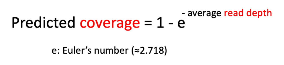
Using this equation, you can predict what average depth your should aim for so that you cover your target sequence at least once (see table below)
| Average Depth | Predicted Coverage |
| 1x | 63.2% |
| 2x | 86.5% |
| 5x | 99.3% |
| 10x | 99.995%s |
YOGI BERRA’S CAVEAT
As in any model, theory and prediction can disagree. The disagreement can lead to overestimating the read depth in certain regions and, as a consequence, overestimating the coverage.
This is because the Lander-Waterman model assumes that your target genome is sequenced randomly—meaning the reads are randomly distributed across the entire length of your target (this is called a Poisson distribution). Of course, the theory rarely reflects the reality of the lab, as technical and biological reasons come in the way
To quote the legendary Yogi Berra:
In theory, between theory and practice there is no difference. In practice, there is.
Every scientist should remember this gem.
MORE MISCONCEPTIONS IN GENOMICS